In the fourth tab, you find Data states (or short “states”) which are the connection for incoming data of a digital twin. Each digital twin can have many states to group data from different sources. Sources can be e.g. data from sensors, aggregated data from other digital twins, or randomly generated data for testing.

Data states are a powerful feature in niotix: With states, you can use digital twins to group different data from the IoT world (e.g. different sensors with different protocols) in a logical container representing a physical object. For e.g. an office can be represented by a digital twin, grouping all the different sensors in each room for humidity and temperature in one place.

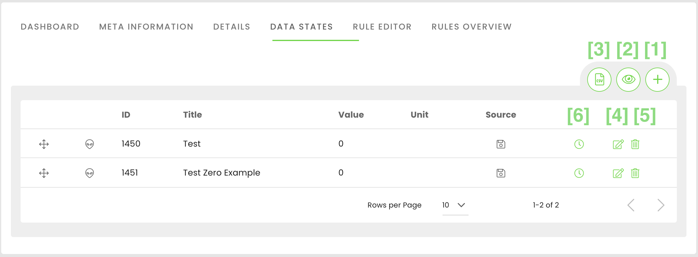
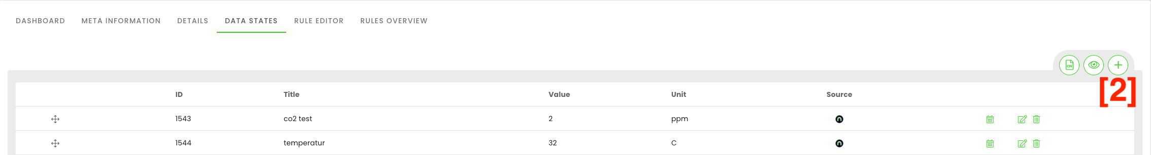
In this tab, you can add a single state [1] or view details of all existing states [2]. You can export the CSV file of the received data of the devices [3].

Furthermore, you can edit [4] and delete [5] each state. By clicking on the “clock”-button, you can see the history of state updates (changed/reported values) [6].

Add single state

If you click on the “+"-button, you can add a single state. Basic settings of a state are:

• Title: title for this state
• Identifier: A key without special characters for identifying this state in the system (must be unique per digital twin). You can use a state to dynamically update the geo-location of a digital twin. By this, a digital twin can represent a mobile asset, and the reported position of a GPS device can update the digital twin. As soon as an identifier starts with “lon” or “lat”, the state will automatically be linked to the longitude- and latitude fields.
• Unit: The unit which is displayed together with the value delivered from this state.
• Icon: An icon for the state. To search for other icons, simply type in a keyword and the system will propose suitable icons.
• Source: Select the bridge defined in your account for incoming data: “Aggregated” to use data from other digital twins or “Random” to generate random data or the bridge configured in your account (e.g. niotix; further description of each source see below).
  • For Connector-Type “MQTT”: With the text fields (Device)Identifier” and “parsed packet variable,” you can define the topic a state should subscribe to on the MQTT broker. The “Device)Identifier” is required, the other value is optional. Both fields are concatenated and must follow the pattern defined in the MQTT-connect in the field “path”.
• Value type: Define the type of the value; e.g. if it is a number, a boolean (true/false) or a string
• Value: Define a default value - which might be overwritten by the incoming data from a selected data source.
• Is null: Mark this checkbox if the value should be empty - not the value “0”!
• Skip transformer: Mark this checkbox if niotix should not run the javascript transformer when you save the state for the first time. Deactivate this switch if you manually set an initial value for a sensor, and you do not want to overwrite it directly with the latest devices’ value (e.g. if the device is not yet installed but activated and thus not measuring the right values)
• Lower bound: The lower bound is used for the visualization on the dashboard to define the limits of e.g. a gauge.
• Upper bound: The upper bound is used for the visualization on the dashboard to define the limits of e.g. a gauge.
• Javascript transformer: Define a transformation function for transforming input data to the desired state value. The transformation will be executed each time the state is updated. See the description below for details.

Source Types

The source of the data point defines where it obtains its data from. Numerous options are available for this, which are described in the following sections:

• Aggregate
• Aggregated timeseries
• Connector
• Dynamical Datarouting
• Iot Data Hub Aggregation
• Random
• Virtual Device
• Virtual Device Aggregation

Visualization

For each data point, you can set different visualizations that will appear in the dashboard and map view. The following visualizations are available:

Standard: If you do not select any other visualization, the counter will appear automatically.
Gauge: Can be used for temperature or light intensity. With a dial gauge, critical limit values are displayed with value specifications and different colors. Define these values using the Minimum value and Maximum value fields as well as one or more comma-separated threshold values. These values are displayed in the dial gauge. You can also define in which colors the values should be displayed.
Donut: This visualization is suitable, among other things, for displaying individual percentage values, e.g. for people counting. In the donut, partial values of a whole are visualized as parts of a circle.
Counter: Can be used for metering. With the counter you can tailor the visualization to your needs: Determine the minimum character length and the decimal places.
Battery: Here the state of charge of e.g. a device is visualized by bars in a battery.
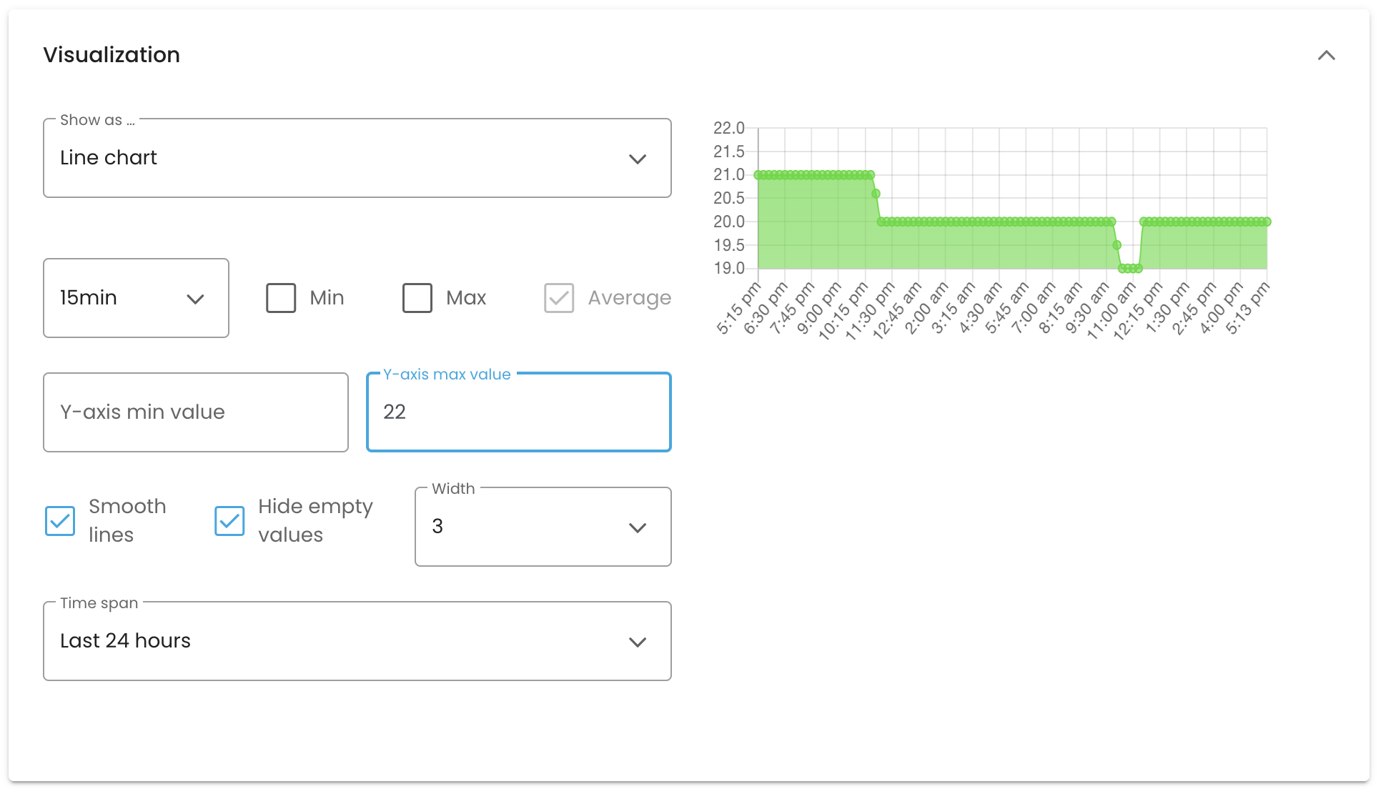
Line chart: The historical data of a data point is displayed in a graph. You can specify the lowest and highest value on the X-axis as well as the time period.

In order to be able to compare several line charts in a dashboard with each other, it can be useful to fix the values of the y-axis. For each chart it is now possible to set a minimum and a maximum value of the y-axis. The y-axis is then fixed in the dashboard. Values above the maximum or below the minimum are cut off in the visualisation. If no minimum or maximum value is defined, the axis remains variable at this section of the axis.

Since a longer period of time is often to be considered in a line chart, it is also helpful to give this visualisation a larger space in the dashboard.

Therefore, it is possible to define the space they take up in the dashboard, as well as the time span and interval to be displayed.

Boolean: With this visualization, it is possible to display truth values. For each state (True or False), a title, an icon, and the color of the icon needs to be selected.

Boolean Button

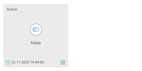
It is possible to create a button in the dashboard of a digital twin that can be used to generate the boolean values True and False to be used in rules and to send downlinks to devices.

This button is a data state with the visualisation for boolean values. Accordingly, it is created as follows: Since the button does not access any data source, the source “none” must be selected and the type “boolean”. It is then possible to select “button” as the visualisation. By saving, the boolean button is created as dashboard tile.

If the status of the boolean button is to be accessed in another data point, this is possible by creating an aggregated state and the following transformer, whereby “button_identifier” must be replaced by the respective key of the data state in which the boolean button was created:

module.exports = (data) => {
 	return data.button_identifier.value;
}

Linking data points with geocoordinates of a twin

To display the history of recorded GPS data from other connectors (not IoT Data Hub) in the map view, you can create the data points according to these instructions:

1. Create two separate data points/states for your Twin, namely Longitude and Latitude. Only one variable can be selected per state.

2. For the dashboard visualization of the two states you can select “hidden”, as they do not necessarily have to be displayed.

3. Create another state of the source “Aggregated” and select the two previously created states for aggregation.

   

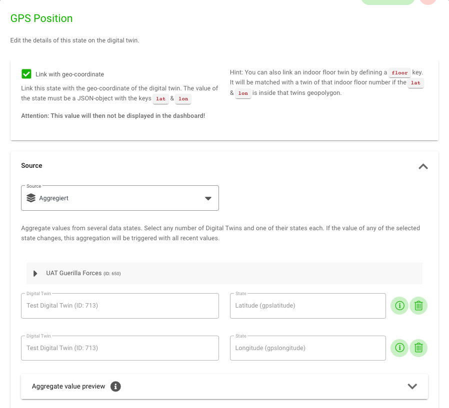
4. Set the state type as “json”.

5. Add the following to the transformer:

module.exports = (data) => {
 	return {lat: data.gpsLatitude, lon: data.gpsLongitude};
}

1. Activate the upper checkbox “Link to geo-coordinate”.

2. Now your twin will be positioned in the map view based on the aggregated data point.

   

Outbound Configuration

To be able to send data to the IEC server, the individual data points must be configured.

• Common Address (ca): The address is called common address because it is connected to all objects contained in the ASDU. Assignment of the Common Address max: 1, min: 65534.

• Information Object Address (ioa): Each information object is addressed by an Information Object Address (IOA), which identifies the respective data within a particular station. Its length is 3 bytes for IEC 104. The address is used as destination address in control direction and as source address in monitoring direction. Assignment of the information object address min: 1, max: 16777215

• Type (data type; type): Here the standard IEC data type must be selected.
  
  Supported types:

  Type Identification	Type Identifier	ASDU Read Type
  1	M_SP_NA	Single-point information
  3	M_DP_NA	Double-point information
  13	M_ME_NC	Short floating point number
  15	M_IT_NA	Integrated totals
  30	M_SP_TB	Single-point -> with time tag
  31	M_DP_TB	Double-point -> with time tag
  36	M_ME_TF	Short floating point number -> with time tag
  37	M_IT_TB	Integrated totals -> with time tag

• Dead Band (db): Sets the threshold for each measured data point. A value change must be greater than the dead band to be reported as an event-driven event. The setting is optional (default value= 0.0) and only relevant for measured values. Permissible types are int and float (e.g. “deadband”: 3.0)

Javascript Transformer

You can define custom transformers to transform incoming data into the desired format and values. To use this powerful feature, basic knowledge of javascript is required.

• Sample scripts: niotix provides some basic javascript as examples of how to work with the transformer. Select one of the examples from the dropdown list to see the javascript code.
• Helper methods: Here you can see a list of often applied and supported javascript libraries that you can use to write transformers. Please have a look at the corresponding documentation of each library.
• Sample value: To test your transformer, you can insert a value here. The button “preview” will use this value as incoming data for the transformer and display the result in the field “transformer result preview”.

In general, the javascript transformer uses a similar annotation to NPM packages. A transformer is handled like a module and needs to explicitly define the exported result (module.exports). You can define the variable name of the incoming data by using the arrow function (...= (IncomingData) => { ... }). You have to return the result with return(TransformedResult)

module.exports = (data) => {
 	return (TransformedResult);
}

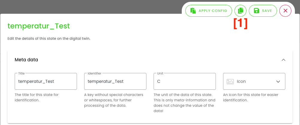
Copying data states from digital twins

Under the digital twins there is also the possibility to copy already created data states and to use its attributes for the new creation of another data state from the same or another twin. This function thus makes it possible to create multiple data states with similar attributes from the same or different (device) sources more easily and quickly.

To copy a data state, first go to the “Edit” icon of the data point you want to copy. In the upper line of the edit view you will find the button “Copy configuration” [1], then click on it and close the window again.

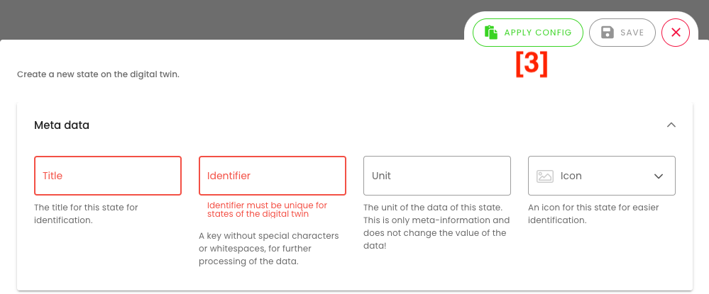
To create a new data state in the same twin or in another twin, click on the plus symbol in the upper right corner [2].

Now click on the button “Apply Config” [3].

A new window will open where all attributes (title, key, unit, visualization, etc.) are already automatically selected for the next step of the transfer. However, you can change the selection of attributes according to your needs. After the selection you click on “Apply configuration”[4].

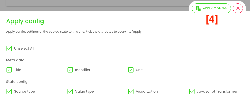
The fields or settings of the new datapoint will now be configured and filled in based on the previously selected information from the original datapoint. Please note that as the last step of the configuration you have to add the data source and possibly change the key (if the same title remains), as this may only occur once for each twin.

SV-Export state history

You can export incoming data from digital twins as CSV-file. To do this easily, click on Data points. By clicking the CSV-icon you can configure the export [1].

When you click on the CSV icon, a new window will open where you can select the time period as well as select the required data points. You can also specify a name and an email address to which a download link will be sent after the download is finished. As soon as you select a data point, you can generate the CSV-file by clicking on the “export” button.

You can find the CSV-file by clicking on the “CSV” button in the top right corner of the menu bar. Then the page “CSV-Export” opens, where you can download the file. Here you can either click directly on the icon located on the right side of the line [2], or you can select the file and click on the download icon.